import numpy as np
import matplotlib.pyplot as plt
%matplotlib inline
Forward pass
input $x$ –> hidden layer 1 unit $q$ –> hidden layer 2 unit $j$ –> output layer unit $k$
(assuming all layers are fully connected, and the activation function is $\sigma$)
Backprop
When we are backpropagating error terms, we go from the output back to the input
output layer unit $k$ –> hidden layer 2 unit $j$ –> hidden layer 1 unit $q$ –> input $x$
Loss function to output layer $L$
\[-\frac{\partial L_{MSE}}{\partial k}=-\frac{\partial L}{\partial \hat{y}}\frac{\partial \hat{y}}{\partial k}=2(y-\hat{y})\sigma'(k)=\delta_k^L\]We use $\delta_k^L$ to represent the error term of node k of last layer L
Output layer L to last hidden layer $L-1$
1. weight update
\[-\frac{\partial L_{MSE}}{\partial w_{jk}}=-\frac{\partial L}{\partial \hat{y}}\frac{\partial \hat{y}}{\partial k}\frac{\partial k}{\partial w_{jk}}= \delta_k^L \sigma(j)\] \[\Delta w_{jk} = \eta \delta_k^L \sigma(j)\]2. error term
\[-\frac{\partial L_{MSE}}{\partial j}=-\frac{\partial L}{\partial \hat{y}}\frac{\partial \hat{y}}{\partial k}\frac{\partial k}{\partial j}=\sum \delta_k^L w_{jk} \sigma'(j)=\delta_j^{L-1}\]$w_{jk}$ is the weight connecting node $j$ in layer $L-1$ to node $k$ in output layer $L$
We use $\delta_j^{L-1}$ to represent the error term of node j of the layer before output layer, which is L-1
Last hidden layer L-1 to previous hidden layer L-2
1. weight update
\[-\frac{\partial L_{MSE}}{\partial w_{qj}}=-\frac{\partial L}{\partial \hat{y}}\frac{\partial \hat{y}}{\partial k}\frac{\partial k}{\partial j}\frac{\partial j}{\partial w_{qj}}= \delta_j^{L-1} \sigma(q)\] \[\Delta w_{qj} = \eta \delta_j^{L-1} \sigma(q)\]2. error term
\[-\frac{\partial L_{MSE}}{\partial q}=-\frac{\partial L}{\partial \hat{y}}\frac{\partial \hat{y}}{\partial k}\frac{\partial k}{\partial j}\frac{\partial j}{\partial q}=\sum \delta_j^{L-1}w_{qj}\sigma'(q) = \delta_q^{L-2}\]$w_{qj}$ is the weight connecting node $q$ in layer $L-2$ to node $j$ in output layer $L-1$
We use $\delta_1^{L-2}$ to represent the error term of node $q$ of the layer $L-2$
Vanishing Gradient
As we backpropagate, we will keep timing $\sigma’(j) = \sigma(j) (1-\sigma(j))$ to the error term.
Here $j$ is the node where we are trying to calculate the error term)
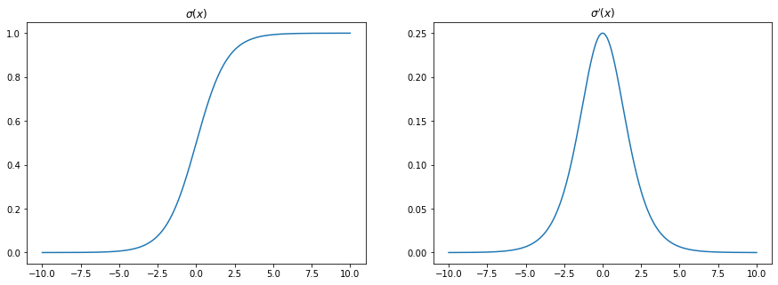
Below is a plot of $\sigma’(x) = \sigma(x) (1-\sigma(x)) = \frac{e^{-x}}{(1+e^{-x})^2}$
We can see that $\max\sigma’(x)=0.25$.
This means, as we go back one layer during backpropagation, the error term is scaled back at least by 75%. If we go two layers back, the error term is scaled back by at least $1-0.25^2=0.9375$
x = np.linspace(-10, 10, 1000)
fig, ax = plt.subplots(1,2, figsize=(15,5))
ax[0].plot(x, 1 / (1+np.exp(-x)))
ax[0].set_title(r'$\sigma(x)$')
ax[1].plot(x, np.exp(-x) / ((1+np.exp(-x)) ** 2))
ax[1].set_title(r"$\sigma'(x)$");
What about hyperbolic tangent?
$\tanh(x) = \frac{e^x-e^{-x}}{e^x+e^{-x}}$
$\tanh’(x) = \frac{4e^{2x}}{(1+e^{2x})^2}$
x = np.linspace(-10, 10, 1000)
fig, ax = plt.subplots(1,2, figsize=(15,5))
ax[0].plot(x, (np.exp(x) - np.exp(-x)) / (np.exp(x) + np.exp(-x)))
ax[0].set_title(r'$\tanh(x)$')
ax[1].plot(x, 4 * np.exp(2*x) / ((1+np.exp(2*x)) ** 2))
ax[1].set_title(r"$\tanh'(x)$");
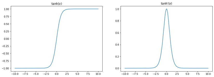
It looks like vanishing gradient is less of a problem with $\tanh$ activation.